The fifth example produces a summary table of selected Vital Signs for Placebo vs. Treated groups. The report shows statistics for both baseline and after-treatment time points. This example also demonstrates how to use tidyverse functions for data preparation instead of procs.
Program
Note the following about this example:
- The
%eq%operator from the common package allows comparing of a variable that contains many NA values, without error. - The fmtr package provides capabilities to create a
user-defined format, similar to
proc format. - The reporter package supports spanning headers in the report header.
- Notice that sassy functions integrate nicely with
dplyr. You can put a
datastep()right in the middle of a dplyr pipeline and get the best of both worlds!
library(tidyverse)
library(sassy)

options("logr.autolog" = TRUE,
        "logr.notes" = FALSE)

# Get path to temp directory
tmp <- tempdir()

# Get path to sample data
pkg <- system.file("extdata", package = "sassy")

# Open log
lgpth <- log_open(file.path(tmp, "example5.log"))

sep("Prepare Data")

# Create libname for csv data
libname(sdtm, pkg, "csv")

put("Join and prepare data")
prep <- sdtm$DM |>
  left_join(sdtm$VS, by = c("USUBJID" = "USUBJID")) |>
  select(USUBJID, VSTESTCD, VISIT, VISITNUM, VSSTRESN, ARM, VSBLFL) |>
  filter(VSTESTCD %in% c("PULSE", "RESP", "TEMP", "DIABP", "SYSBP"),
         !(VISIT == "SCREENING" & VSBLFL != "Y")) |>
  arrange(USUBJID, VSTESTCD, VISITNUM) |>
  group_by(USUBJID, VSTESTCD) |>
  datastep(retain = list(BSTRESN = 0), {

    # Combine treatment groups
    # And distingish baseline time points
    if (ARM == "ARM A") {
      if (VSBLFL %eq% "Y") {
        GRP <- "A_BASE"
      } else {
        GRP <- "A_TRT"
      }
    } else {
      if (VSBLFL %eq% "Y") {
        GRP <- "O_BASE"
      } else {
        GRP <- "O_TRT"
      }
    }

    # Populate baseline value
    if (first.)
      BSTRESN = VSSTRESN

  }) |>
  ungroup()

put("Get population counts")
pop_A <- prep |> select(USUBJID, GRP) |> filter(GRP == "A_BASE") |>
  distinct() |> count() |> deframe() |> put()
pop_O <- prep |> select(USUBJID, GRP) |> filter(GRP == "O_BASE") |>
  distinct() |> count() |> deframe() |> put()

put("Prepare final data frame")
final <- prep |>
  select(VSTESTCD, GRP, VSSTRESN, BSTRESN) |>
  group_by(VSTESTCD, GRP) |>
  summarize(Mean = fmt_mean_sd(VSSTRESN),
            Median = fmt_median(VSSTRESN),
            Quantiles = fmt_quantile_range(VSSTRESN),
            Range = fmt_range(VSSTRESN)) |>
  ungroup() |>
  pivot_longer(cols = c(Mean, Median, Quantiles, Range),
               names_to = "stats",
               values_to = "values") |>
  pivot_wider(names_from = GRP,
              values_from = values) |>
  put()


sep("Create formats")

# Vital sign lookup format
vs_fmt <- c(PULSE = "Pulse",
            TEMP = "Temperature °C",
            RESP = "Respirations/min",
            SYSBP = "Systolic Blood Pressure",
            DIABP = "Diastolic Blood Pressure") |>
  put()

# Statistics user-defined format
stat_fmt <- value(condition(x == "Mean", "Mean (SD)"),
                  condition(x == "Quantiles", "Q1 - Q3")) |>
  put()

sep("Create Report")


# Apply sort
final <- final |>
  mutate(VSTESTCD = factor(VSTESTCD, levels = names(vs_fmt))) |>
  arrange(VSTESTCD)

# Define table object
tbl <- create_table(final, borders = "bottom") |>
  spanning_header(A_BASE, A_TRT, "Placebo", n = pop_A) |>
  spanning_header(O_BASE, O_TRT, "Treated", n = pop_O) |>
  column_defaults(width = 1.25, align = "center") |>
  stub(c(VSTESTCD, stats), width = 2.5) |>
  define(VSTESTCD, "Vital Sign", format = vs_fmt,
         blank_after = TRUE, dedupe = TRUE, label_row = TRUE) |>
  define(stats, indent = .25, format = stat_fmt) |>
  define(A_BASE, "Baseline") |>
  define(A_TRT, "After Treatment") |>
  define(O_BASE, "Baseline") |>
  define(O_TRT, "After Treatment")

# Construct output path
pth <- file.path(tmp, "output/t_vs.pdf")

# Define report object
rpt <- create_report(pth, output_type = "PDF", font = "Times",
                     font_size = 11) |>
  page_header("Sponsor: Company", "Study: ABC") |>
  titles("Table 4.0", "Selected Vital Signs", bold = TRUE, font_size = 12) |>
  add_content(tbl, align = "center") |>
  page_footer(Sys.time(), "CONFIDENTIAL", "Page [pg] of [tpg]")

# Write report to file system
write_report(rpt)

# Close log
log_close()

# View files
# file.show(pth)
# file.show(lgpth)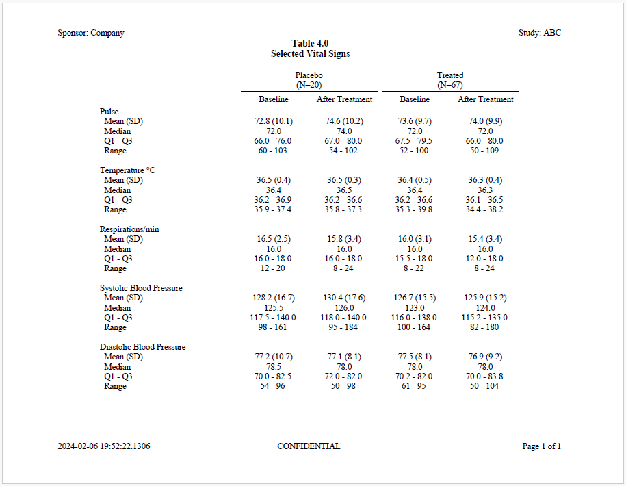
Log
Here is the log from the above example:
=========================================================================
Log Path: C:/Users/User/AppData/Local/Temp/Rtmpum5T6o/log/example5.log
Working Directory: C:/packages/Testing
User Name: User
R Version: 4.0.3 (2020-10-10)
Machine: DESKTOP-1F27OR8 x86-64
Operating System: Windows 10 x64 build 18363
Log Start Time: 2021-01-05 08:13:13
=========================================================================

=========================================================================
Prepare Data
=========================================================================

# library 'sdtm': 8 items
- attributes: csv not loaded
- path: C:/Users/User/Documents/R/win-library/4.0/sassy/extdata
- items:
  Name Extension Rows Cols     Size        LastModified
1   AE       csv  150   27  88.1 Kb 2020-12-27 23:21:55
2   DA       csv 3587   18 527.8 Kb 2020-12-27 23:21:55
3   DM       csv   87   24  45.2 Kb 2020-12-27 23:21:55
4   DS       csv  174    9  33.7 Kb 2020-12-27 23:21:55
5   EX       csv   84   11    26 Kb 2020-12-27 23:21:55
6   IE       csv    2   14    13 Kb 2020-12-27 23:21:55
7   SV       csv  685   10  69.9 Kb 2020-12-27 23:21:55
8   VS       csv 3358   17   467 Kb 2020-12-27 23:21:55

Join and prepare data

left_join: added 18 columns (STUDYID.x, DOMAIN.x, STUDYID.y, DOMAIN.y, VSSEQ, …)

           > rows only in x       0

           > rows only in y  (    0)

           > matched rows     3,358    (includes duplicates)

           >                 =======

           > rows total       3,358

select: dropped 33 variables (STUDYID.x, DOMAIN.x, SUBJID, RFSTDTC, RFENDTC, …)

filter: removed 590 rows (18%), 2,768 rows remaining

group_by: 2 grouping variables (USUBJID, VSTESTCD)

datastep: columns decreased from 7 to 9

ungroup: no grouping variables

# A tibble: 2,768 x 9
   USUBJID    VSTESTCD VISIT   VISITNUM VSSTRESN ARM   VSBLFL BSTRESN GRP
   <chr>      <chr>    <chr>      <dbl>    <dbl> <chr> <chr>    <dbl> <chr>
 1 ABC-01-049 DIABP    DAY 1          1       76 ARM D Y           76 O_BASE
 2 ABC-01-049 DIABP    WEEK 2         2       66 ARM D <NA>        76 O_TRT
 3 ABC-01-049 DIABP    WEEK 4         4       84 ARM D <NA>        76 O_TRT
 4 ABC-01-049 DIABP    WEEK 6         6       68 ARM D <NA>        76 O_TRT
 5 ABC-01-049 DIABP    WEEK 8         8       80 ARM D <NA>        76 O_TRT
 6 ABC-01-049 DIABP    WEEK 12       12       70 ARM D <NA>        76 O_TRT
 7 ABC-01-049 DIABP    WEEK 16       16       70 ARM D <NA>        76 O_TRT
 8 ABC-01-049 PULSE    DAY 1          1       84 ARM D Y           84 O_BASE
 9 ABC-01-049 PULSE    WEEK 2         2       84 ARM D <NA>        84 O_TRT
10 ABC-01-049 PULSE    WEEK 4         4       76 ARM D <NA>        84 O_TRT
# ... with 2,758 more rows

Get population counts

select: dropped 7 variables (VSTESTCD, VISIT, VISITNUM, VSSTRESN, ARM, …)

filter: removed 2,669 rows (96%), 99 rows remaining

distinct: removed 79 rows (80%), 20 rows remaining

count: now one row and one column, ungrouped

[1] 20

select: dropped 7 variables (VSTESTCD, VISIT, VISITNUM, VSSTRESN, ARM, …)

filter: removed 2,435 rows (88%), 333 rows remaining

distinct: removed 266 rows (80%), 67 rows remaining

count: now one row and one column, ungrouped

[1] 67

Prepare final data frame

select: dropped 5 variables (USUBJID, VISIT, VISITNUM, ARM, VSBLFL)

group_by: 2 grouping variables (VSTESTCD, GRP)

summarize: now 20 rows and 6 columns, one group variable remaining (VSTESTCD)

ungroup: no grouping variables

pivot_longer: reorganized (Mean, Median, Quantiles, Range) into (stats, values) [was 20x6, now 80x4]

pivot_wider: reorganized (GRP, values) into (A_BASE, A_TRT, O_BASE, O_TRT) [was 80x4, now 20x6]

# A tibble: 20 x 6
   VSTESTCD stats     A_BASE        A_TRT         O_BASE        O_TRT
   <chr>    <chr>     <chr>         <chr>         <chr>         <chr>
 1 DIABP    Mean      77.2 (10.7)   77.1 (8.1)    77.5 (8.1)    76.9 (9.2)
 2 DIABP    Median    78.5          78.0          78.0          78.0
 3 DIABP    Quantiles 70.0 - 82.5   72.0 - 82.0   70.2 - 82.0   70.0 - 83.8
 4 DIABP    Range     54 - 96       50 - 98       61 - 95       50 - 104
 5 PULSE    Mean      72.8 (10.1)   74.6 (10.2)   73.6 (9.7)    74.0 (9.9)
 6 PULSE    Median    72.0          74.0          72.0          72.0
 7 PULSE    Quantiles 66.0 - 76.0   67.0 - 80.0   67.5 - 79.5   66.0 - 80.0
 8 PULSE    Range     60 - 103      54 - 102      52 - 100      50 - 109
 9 RESP     Mean      16.5 (2.5)    15.8 (3.4)    16.0 (3.1)    15.4 (3.4)
10 RESP     Median    16.0          16.0          16.0          16.0
11 RESP     Quantiles 16.0 - 18.0   16.0 - 18.0   15.5 - 18.0   12.0 - 18.0
12 RESP     Range     12 - 20       8 - 24        8 - 22        8 - 24
13 SYSBP    Mean      128.2 (16.7)  130.4 (17.6)  126.7 (15.5)  125.9 (15.2)
14 SYSBP    Median    125.5         126.0         123.0         124.0
15 SYSBP    Quantiles 117.5 - 140.0 118.0 - 140.0 116.0 - 138.0 115.2 - 135.0
16 SYSBP    Range     98 - 161      95 - 184      100 - 164     82 - 180
17 TEMP     Mean      36.5 (0.4)    36.5 (0.3)    36.4 (0.5)    36.3 (0.4)
18 TEMP     Median    36.4          36.5          36.4          36.3
19 TEMP     Quantiles 36.2 - 36.9   36.2 - 36.6   36.2 - 36.6   36.1 - 36.5
20 TEMP     Range     35.9 - 37.4   35.8 - 37.3   35.3 - 39.8   34.4 - 38.2

=========================================================================
Create formats
=========================================================================

PULSE                       TEMP                       RESP                      SYSBP
"Pulse"           "Temperature °C"         "Respirations/min"  "Systolic Blood Pressure"
DIABP
"Diastolic Blood Pressure"

# A user-defined format: 2 conditions
  Name Type       Expression     Label Order
1    x    U      x == "Mean" Mean (SD)    NA
2    x    U x == "Quantiles"   Q1 - Q3    NA

=========================================================================
Create Report
=========================================================================

mutate: converted 'VSTESTCD' from character to factor (0 new NA)

# A report specification: 1 pages
- file_path: 'C:\Users\User\AppData\Local\Temp\Rtmpum5T6o/output/t_vs.rtf'
- output_type: RTF
- units: inches
- orientation: landscape
- line size/count: 108/48
- page_header: left=Sponsor: Company right=Study: ABC
- title 1: 'Table 4.0'
- title 2: 'Selected Vital Signs'
- page_footer: left=2021-01-05 08:13:45 center=CONFIDENTIAL right=Page [pg] of [tpg]
- content:
# A table specification:
- data: tibble 'final' 20 rows 6 cols
- show_cols: all
- use_attributes: all
- spanning_header: from='A_BASE' to='A_TRT' 'Placebo' level=1
- spanning_header: from='O_BASE' to='O_TRT' 'Treated' level=1
- stub: VSTESTCD stats width=2.5 align='left'
- define: VSTESTCD 'Vital Sign' dedupe='TRUE'
- define: stats
- define: A_BASE 'Baseline'
- define: A_TRT 'After Treatment'
- define: O_BASE 'Baseline'
- define: O_TRT 'After Treatment'

=========================================================================
Log End Time: 2021-01-05 08:13:49
Log Elapsed Time: 0 00:00:36
=========================================================================