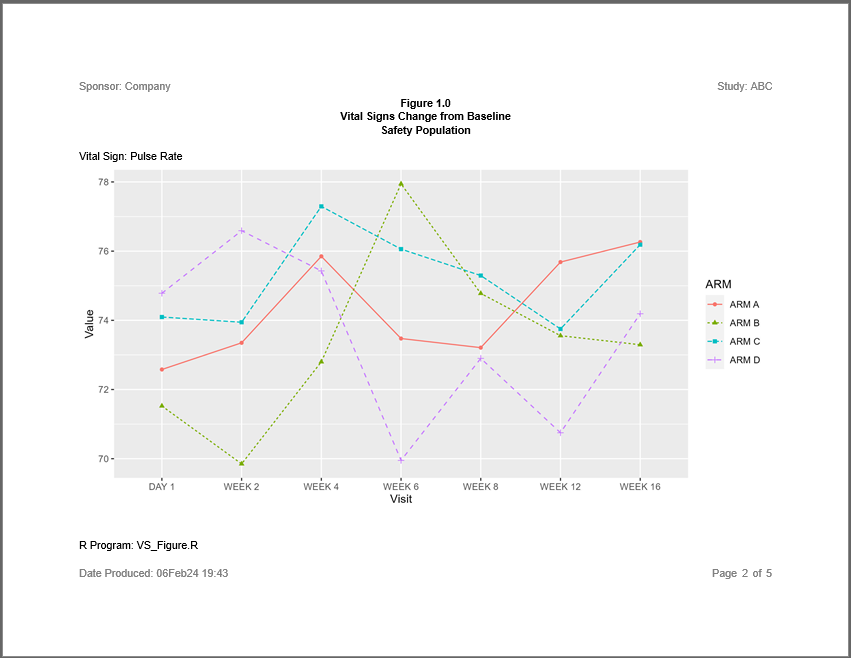
The sassy system gives you capabilities that few other R packages can match. The system not only support reports with by-groups. You can even apply a by-group to a figure.
Program
Note the following about this example:
- The plot is created as a single plot with no by-groups
- The plot is added to the report with the
add_content()function, just like the figures in the previous example. - The
page_by()function on thecreate_plot()statement generates the paging for both the report and plot.
library(sassy)
library(ggplot2)

options("logr.autolog" = TRUE,
        "logr.notes" = FALSE)

# Get path to temp directory
tmp <- tempdir()

# Get path to sample data
pkg <- system.file("extdata", package = "sassy")

# Open log
lgpth <- log_open(file.path(tmp, "example6.log"))

# Prepare Data ------------------------------------------------------------

sep("Prepare Data")

put("Load data files")
libname(dat, pkg, "csv", filter = c("DM", "VS"))


put("Prepare factor levels")
visit_levels <- c("SCREENING", "DAY 1",   "WEEK 2",  "WEEK 4",  "WEEK 6",
                  "WEEK 8",  "WEEK 12", "WEEK 16") |> put()

arm_levels <- c("ARM A", "ARM B") |> put()

test_codes <- c("SYSBP", "DIABP", "PULSE", "RESP") |> put()

put("Prepare data for analysis")
datastep(dat$DM, merge = dat$VS, merge_by = v(STUDYID, USUBJID),
         keep = v(STUDYID, USUBJID, ARM, VISIT, VSTESTCD, VSORRES),
         merge_in = v(inDM, inVS),
         where = expression(VISIT != "END OF STUDY EARLY TERMINATION" &
                            ARM %in% c("ARM A", "ARM B") &
                            VSTESTCD %in% test_codes
                            ),
         {

           # Assign factors to VISIT and ARM
           VISIT <- factor(VISIT, levels = visit_levels)
           ARM <- factor(ARM, levels = arm_levels)
           VSTESTCD <- factor(VSTESTCD, levels = test_codes)

           if (!inDM & inVS) {
             delete()
           }

         }) -> vitals


# Create Plot -------------------------------------------------------------

sep("Create Plot")

put("Assign Colors")
arm_cols <- c("ARM B" = "#1f77b4", "ARM A" = "#2f2f2f")

put("Define Boxplot")
p_box <- ggplot2::ggplot(
  vitals,
  ggplot2::aes(x = VISIT, y = VSORRES, fill = ARM, colour = ARM)
) +
  ggplot2::geom_boxplot(
    position = ggplot2::position_dodge(width = 0.75),
    width = 0.6,
    outlier.size = 0.7,
    alpha = 0.9
  ) +
  ggplot2::scale_fill_manual(values = arm_cols) +
  ggplot2::scale_colour_manual(values = arm_cols) +
  ggplot2::labs(
    x = NULL,
    y = "Lab Value",
    fill = NULL,
    colour = NULL
  ) +
  ggplot2::theme_bw(base_size = 10) +
  ggplot2::theme(
    legend.position = "bottom",
    panel.grid.major.x = ggplot2::element_blank(),
    plot.title = ggplot2::element_text(face = "bold", hjust = 0),
    plot.caption = ggplot2::element_text(hjust = 0)
  )

put("Create format for lab codes")
lbfmt <- value(condition(x == "SYSBP", "Systolic Blood Pressure (mmHg)"),
               condition(x == "DIABP", "Diastolic Blood Pressure (mmHg)"),
               condition(x == "PULSE", "Pulse (bpm)"),
               condition(x == "RESP", "Respirations (bpm)"))


# Report ------------------------------------------------------------------

sep("Report")

put("Create plot object definition")
plt <- create_plot(p_box, height = 4, width = 7, borders = "outside") |>
  titles("Figure 10. Box Plot: Median and Interquartile Range of Vital Signs by Treatment Arm",
         bold = TRUE, font_size = 12, align = "left") |>
  page_by(VSTESTCD, label = "Lab Test: ", format = lbfmt, blank_row = "none") |>
  footnotes(
    "Source: example6.rtf. {version$version.string}",
    "Note: Boxes span the interquartile range (25th to 75th percentile); horizontal line = median;",
    "whiskers = 1.5×IQR; individual outliers are those beyond this range.",
    font_size = 9, italics = TRUE, blank_row = "none"
  )

put("Create report output path")
pth <- file.path(tempdir(), "example6.rtf")

put("Create report")
rpt <- create_report(pth, font = "Arial", font_size = 10, output_type = "RTF") |>
  page_header("Sponsor: Company", right = "Study: ABC", blank_row = "below") |>
  add_content(plt) |>
  page_footer("Date Produced: {fapply(Sys.Date(), 'date7')}", right = "Page [pg] of [tpg]")

put("Write report to file system")
write_report(rpt)

put("Close log")
log_close()

# View report
# file.show(pth)

# View log
# file.show(lgpth)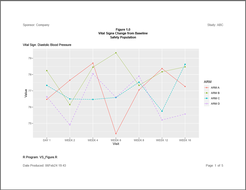
Log
Here is the log for the above program:
=========================================================================
Log Path: C:/Users/dbosa/AppData/Local/Temp/Rtmpq0yZA5/log/example6.log
Program Path: C:/Studies/Testing1/P6b.R
Working Directory: C:/Studies/Testing1
User Name: dbosa
R Version: 4.4.3 (2025-02-28 ucrt)
Machine: SOCRATES x86-64
Operating System: Windows 10 x64 build 26100
Base Packages: stats graphics grDevices utils datasets methods base
Other Packages: tidylog_1.1.0 ggplot2_3.5.1 procs_1.0.7 reporter_1.4.5
libr_1.3.9 logr_1.3.9 fmtr_1.7.0 common_1.1.4 sassy_1.2.9
Log Start Time: 2025-12-12 14:27:32.328372
=========================================================================

=========================================================================
Prepare Data
=========================================================================

Load data files

# library 'dat': 2 items
- attributes: csv not loaded
- path: C:/Users/dbosa/AppData/Local/R/win-library/4.4/sassy/extdata
- items:
  Name Extension Rows Cols     Size        LastModified
1   DM       csv   87   24  45.8 Kb 2025-12-12 08:37:33
2   VS       csv 3358   17 467.7 Kb 2025-12-12 08:37:33

Prepare factor levels

SCREENING
DAY 1
WEEK 2
WEEK 4
WEEK 6
WEEK 8
WEEK 12
WEEK 16

ARM A
ARM B

SYSBP
DIABP
PULSE
RESP

Prepare data for analysis

datastep: columns decreased from 24 to 6

# A tibble: 1,231 × 6
   STUDYID USUBJID    ARM   VISIT     VSTESTCD VSORRES
   <chr>   <chr>      <fct> <fct>     <fct>      <dbl>
 1 ABC     ABC-01-050 ARM B SCREENING DIABP         80
 2 ABC     ABC-01-050 ARM B DAY 1     DIABP         78
 3 ABC     ABC-01-050 ARM B WEEK 2    DIABP         64
 4 ABC     ABC-01-050 ARM B WEEK 4    DIABP         86
 5 ABC     ABC-01-050 ARM B WEEK 6    DIABP         70
 6 ABC     ABC-01-050 ARM B WEEK 8    DIABP         80
 7 ABC     ABC-01-050 ARM B WEEK 12   DIABP         64
 8 ABC     ABC-01-050 ARM B WEEK 16   DIABP         82
 9 ABC     ABC-01-050 ARM B SCREENING PULSE         76
10 ABC     ABC-01-050 ARM B DAY 1     PULSE         68
# ℹ 1,221 more rows
# ℹ Use `print(n = ...)` to see more rows

=========================================================================
Create Plot
=========================================================================

Assign Colors

Define Boxplot

Create format for lab codes

# A user-defined format: 4 conditions
  Name Type   Expression                           Label Order
1  obj    U x == "SYSBP"  Systolic Blood Pressure (mmHg)    NA
2  obj    U x == "DIABP" Diastolic Blood Pressure (mmHg)    NA
3  obj    U x == "PULSE"                     Pulse (bpm)    NA
4  obj    U  x == "RESP"              Respirations (bpm)    NA

=========================================================================
Report
=========================================================================

Create plot object definition

Create report output path

Create report

Write report to file system

# A report specification: 4 pages
- file_path: 'C:\Users\dbosa\AppData\Local\Temp\Rtmpq0yZA5/example6.rtf'
- output_type: RTF
- units: inches
- orientation: landscape
- margins: top 0.5 bottom 0.5 left 1 right 1
- line size/count: 9/42
- page_header: left=Sponsor: Company right=Study: ABC
- page_footer: left=Date Produced: 12DEC25 center= right=Page [pg] of [tpg]
- content:
# A plot specification:
- data: 1231 rows, 6 cols
- layers: 1
- height: 4
- width: 7
- page by: VSTESTCD
- title 1: 'Figure 10. Box Plot: Median and Interquartile Range of Vital Signs by Treatment Arm'
- footnote 1: 'Source: example6.rtf. R version 4.4.3 (2025-02-28 ucrt)'
- footnote 2: 'Note: Boxes span the interquartile range (25th to 75th percentile); horizontal line = median;'
- footnote 3: 'whiskers = 1.5×IQR; individual outliers are those beyond this range.'

Close log

=========================================================================
Log End Time: 2025-12-12 14:27:40.667776
Log Elapsed Time: 0 00:00:08
=========================================================================